
This is a summary of my first empirical work, my Master’s thesis in economics: Mutasci, F. (2019). “The Impact of Pollution on Property Price Evaluation: A Spatial Approach to Hedonic Pricing Models”, University of Milan.
Summary
The purpose of the study is to investigate one of the problems affecting the economy of the city of Taranto, namely the possibility that the deposit of polluting particulate matter (PM10) related to the presence of the former ILVA\ArcelorMittal steelworks exacerbates the decline in property values in working-class neighborhoods. The study uses a set of geolocated data on houses for sale with corresponding hedonic characteristics, including pollution levels estimated using IDW interpolation of ARPA weather station samples, controlling for socioeconomic variables. The research design enriches classic hedonic pricing models through the use of spatial lag matrices, estimating SAR and SEM models with the maximum likelihood method, showing that, although higher concentration of pullutant particles predicts a drop in property price, the devaluation of houses for sale appears to be mainly confined to the suburban neighborhood called “Tamburi”, located next to the steel mill.
Project Aims and Relevance
The methods adopted are part of the rich economic literature on Hedonic Pricing Models (Rosen, 1974). The models estimated also include controls that are not strictly related to the endogenous characteristics of houses – such as the socioeconomic conditions in which real estate properties are located, environmental characteristics and pollution levels – that are treated as determinants of property values, following a methodological framework that is not new in the literature (Henning & Ridker, 1969; Yusufa & Resosudarmo, 2009). Moreover, the research design makes use of SAR and SEM Spatial Models (Anselin, 1999; Martin, 1974; LeSage, 2008; Anselin, 1988; LeSage, 2004) to account for spatial autocorrelation.
The topic of the research in the master’s thesis is part of a heated debate on the problematic relationship between the city of Taranto and the big adjacent steel district (Francesca, et al., 2012; ANSA, 2022; V.N., 2019; PeaceLink, 2007), although only focusing on real estate. Although it is a powerful tool, spatial analyses has never been adopted before to highlight how the most polluted neighborhoods and/or those that are close to the exILVA/ArcelorMittal steelworks also seem to be affected by a major problem of property price depreciation. This analytical framework could certainly be readapted to study the real estate market in other Italian and European cities adjacent to highly polluting factories or industrial complexes – in fact, in Italy alone there should be about 60 other factories interested by critical public debate similar to what happens with the ex-ILVA steel mill in Taranto (EEA, 2011).
Project Description
Data Collection and Compilation of the Dataset
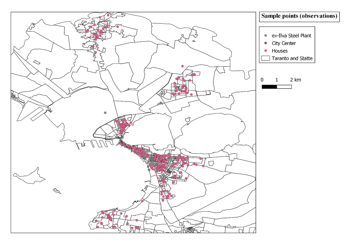
The study makes use of a cross-sectional dataset of houses for sale in the city of Taranto and the neighboring municipality of Statte (which was part of the municipal territory until June 1992), with all observations being geolocated and provided with a set of their characteristics (location, size, number of rooms, energy efficiency class etc.). The working dataset was compiled by:
a) Estimating the concentration of PM10 polluting particles in the air (\(P_{xy}\), mostly caused by industrial activity) over the area of analysis, performing an Inverse Distance Weighted (IDW) Interpolation (Shepard, 1968; Mesnard, 2011; Gimond, 2022) of pollution levels recorded at ARPA monitoring stations (ARPA Puglia; ASL Puglia; AReSS Puglia, 2021):
$$ P_{xy} = \frac{\sum_{i=1}^n w_i p_i}{\sum_{i=1}^n w_i} $$
\(𝑥, 𝑦\) being longitude and latitude of each point \(𝑖\), \(𝑤_𝑖 = |𝑥𝑦_{−𝑖} − 𝑥𝑦_𝑖|^{−𝛼} \) being the inverse of the distance, weighted for the inverse distance power \(𝛼 \geq 0 \) (here \(𝛼 = 2\) as QGIS default settings). The recorded amount of PM10 polluting particles is taken as the mean annual averages from 2016 to 2019, before and after the sale of the steel plant from the previous management of Riva Group to ArcelorMittal. This method of handling the data on pollution also allows to rule out the year-specific biases in the measurements due to particular weather conditions, such as Sahara sandstorms.
b) Computing a sub-local measure of the percentage of residents with a university degree making use of ISTAT census datasets, to be used as an proxy of the socioeconomic conditions of neighborhoods.
c) Collecting a random sample of 428 houses for sale in Taranto with respective characteristics (to be used as hedonic price prectors) from sales advertisements on the websites of the real estate agencies.
Each house was geolocated with a pair of coordinates derived from the address mentioned in sales advertisements. The location of the houses was used to compute the distance of each observation from the city center and from the steel mill (also treated as determinants of selling prices), and hence to match each house with (I) the estimated PM10 levels in the location, (II) the percentage of residents with a university degree in the area of the building.
Preliminary Analyses
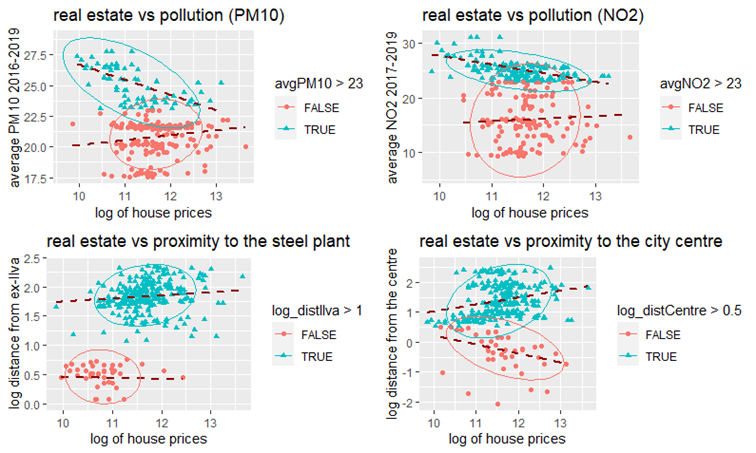
The existence of some kind of nexus between industrial-related pollution/proximity to the industrial district and real estate is roughly identified through various data visualization tools. A first correlation emerges in the scatterplots of Figure 2 between the logarithm of house prices and:
a) The the distance of the houses from the former ILVA (taken as a logarithm to capture
nonlinearity)
b) Average estimated levels of PM10 polluting particles in the position of each one of the houses for sale of the working dataset
The point clouds in Figure 2 seem to descriptively highlight two clusters of distributions. There is a split between the distribution of the prices of houses for sale at high PM10 levels (set as above 23 μg/m3, still below the legal limit threshold of 50 μg/m3) – with prices falling with higher levels of pollution – and that of houses for sale interested by lower average pollution levels. A second, considerably more noticeable family of clusters appears to involve a split between houses that are within 2.7 kilometers - i.e., within the distance where the Tamburi neighborhood is located- from the ex-ILVA steel mill (with lower average prices) and all others. Creating dummy variable that divides the houses located in the Tamburi district from those in the rest of the city, it is in fact possible to show in the Boxplots two distinct price bands, with houses for sale in the Tamburi neighborhood having both lower average prices and a lower price range.
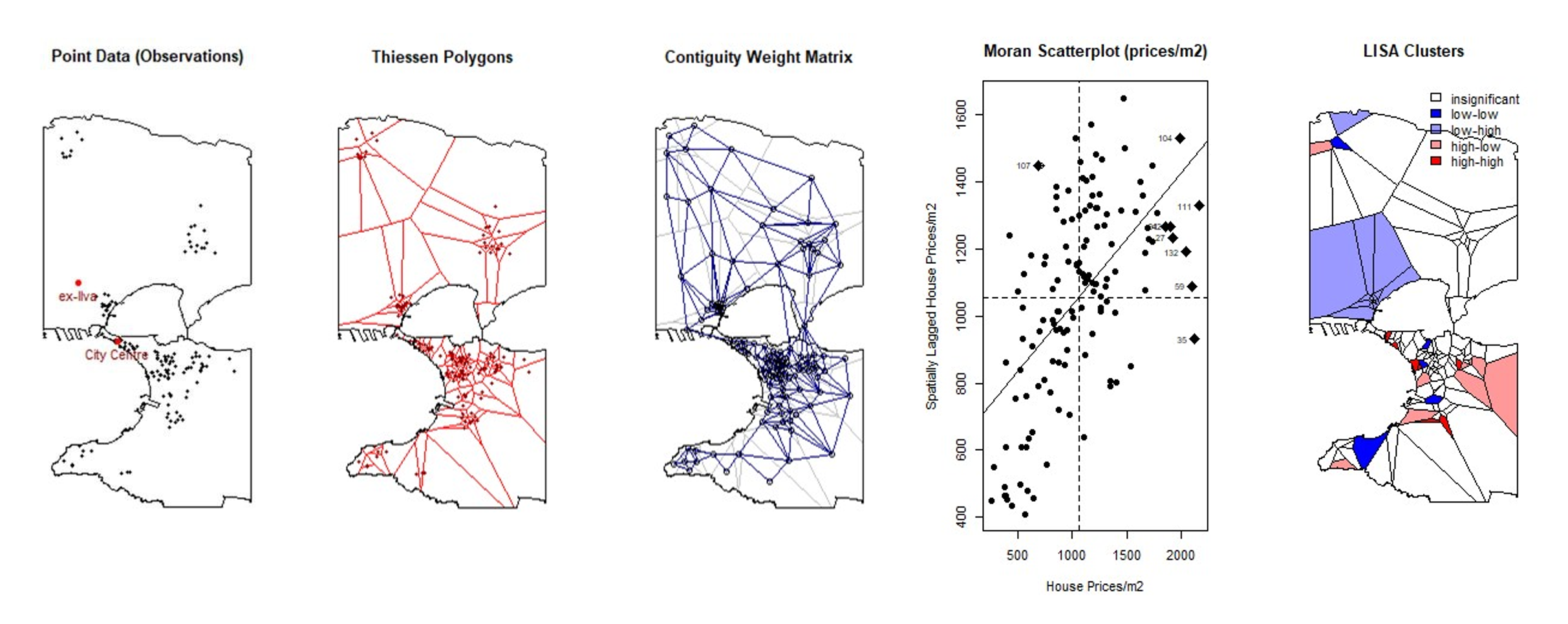
The idea that the Tamburi district represents a cluster of particularly depreciated real estate properties is then further explored through preliminary spatial analyses. Starting from the geospatial position of the houses in the dataset, the area under analysis was divided into Thiessen polygons with each of the observations as centroids, through a Voronoi tessellation (Burrough, McDonnell, & Lloyd, 2008; Longley, Goodchild, Maguire, & Rhind, 2005; Zekai, 2016; Jonathan, s.d.). The polygons obtained were then used to build a Contiguity Weight Matrix (𝑊) (Martin, 1974), defining the neighborhood set of each observation/polygon as the set of all of those observations/polygons with which it shares a side or an edge (Queen contiguity criterion) (Anselin, 2020; Ignacio, 2016).
To check for spatial autocorrelation between the data in the dependent variable, a Moran Scatterplot (Mendez, 2020) is plotted in Figure 3 using the previously defined adjacency matrix, showing a correlation between the prices per square meter of the houses (accounting therefore for the hidden variable of “house size” in the univariate correlation) and the mean squared price in their neighborhood set. The statistically significant spatial clusters and spatial outliers are thus plotted on a map of the LISA Clusters (ibid.) in Figure 3, revealing that the Tamburi district consists of a low-high type spatial outlier – i.e., the areas immediately adjacent to the steel mill are interested by lower-than-average prices per square meter, despite having houses with higher-than-average prices in their proximity set. Interestingly, the city center (from which both the Tamburi district and the steel mill are visible to the naked eye) constitutes a high-high type spatial cluster, highlighting a marked divide from the Tamburi district.
Spatial Regressions
The evidence gathered in preliminary analyses is then tested in hedonic pricing regression models that account for the existence of spatial spillovers, to avoid spatial biases in the resulting estimates. The hypothesis that a higher concentration of pollutant particles in the air and a major proximity to the steel plant leads to a reduction in the expected prices of houses for sale is tested, all other characteristics of the properties for sale being equal, using PM10 levels and the location of the houses in Tamburi district as hedonic determinants of prices in a series of SAR and SEM models – SAR models 1.1-1.3 and SEM models 2.1-2.3, estimated by Maximum Likelihood. The sub-locale percentage of residents with a university degree is included as an additional predictor to control for the socioeconomic conditions in the location where each of the observations is placed.
Spatial regression models are built using a spatial lag operator, i.e., a \(N \times N\) spatial weight matrix 𝑊 which defines set of neighboring positions:
$$ W = \begin{bmatrix} w_{11} & w_{12} & \dots & w_{1n} \\ w_{21} & w_{22} & \dots & w_{2n} \\ \vdots & \vdots & \ddots & \vdots \\ w_{n1} & w_{n2} & \dots & w_{nn} \end{bmatrix} $$
$$ w_{ij} = \frac{w_{ij}^\ast}{\sum_j w_{ij}^\ast} $$
With \(w_{ij}^\ast = 1\) if \(i\) and \(j\) are neighbors (i.e., if they are one spatial lag apart from each other’s), \(w_{ij}^\ast = 0\) otherwise. The spatial lag operator 𝑊 can be modelled in the regression equation in two different ways (Anselin, 1988), to obtain:
- SAR – Spatial Autoregressive Models
If the spatial weight matrix is incorporated into the equation in the form of the regressor 𝑊𝑦 - accounting for spatial autocorrelation in the dependent variable
$$ y = \rho Wy + X_i\beta + e $$
- SEM – Spatial Error Models
If the spatial weight matrix is added instead in the error term, in the form of a non-random spatial disturbance 𝑊\(\epsilon\)
$$ y = + X_i\beta + \epsilon $$
with
$$ E[\epsilon_i \epsilon_j] \neq 0; \ \epsilon = \lambda W + e $$
y being a vector of house prices, 𝑋 a vector of predictors of prices, 𝛽 the coefficient that measures the effect of changes in the value predictors on the dependent variable, 𝜌,𝜆 the coefficients of spatial autocorrelation and spatial disturbance respectively. The term 𝑒 is the vector of non-systematic errors.
Results
Three preliminary specifications of SAR and SEM models were estimated in Tables 1 and 2:
a) Models SAR 1.1 and SEM 2.1, in which main predictor of interest is the level of PM10 pollutant particles
b) Models SAR 1.3 and SEM 2.3, in which the dummy variable of the Tamburi district (neighborhood-specific proxy of the proximity to the steel mill) is used instead, and
c) Models SAR 1.2 and SEM 2.2, two control models in which neither of the previous two predictors is included, with an additional geolocation variable (distance from the city center), to check whether the magnitude of the spatial autocorrelation and spatial disturbance coefficients changes once none of the effects of the predictors related to the presence of the ex-ILVA steel mill is estimated.
The dummy “Tamburi” is found to always have a statistically significant negative effect on expected prices, capturing the influence of proximity to ex-ILVA. The level of PM10 pollutant particles, on the other hand, is only significant in SEM 2.3. In SAR models, the impact of the spatial autocorrelation coefficient 𝜌 is almost doubled in the regression that includes PM10 levels compared to the one with the dummy Tamburi; while in SEM models, the spatial disturbance 𝜆 is not significant in conjunction with said dummy variable. The parameters 𝜆 and 𝜌 are also big in magnitudes in the control regression with distance from the center as geolocational variable, without direct measures of proximity to the ex-ILVA steel mill and industrial pollution. These findings might suggest that in those models where the Tamburi dummy is not present as a predictor, the clustering of prices at the neighborhood level is at least partially captured by the spatial autocorrelation and spatial disturbance coefficients.
Furthermore, the fact that the proxyfor socio-economic conditions (the percentage of residents with a university degree) is always statistically significant, as well as the dummy variable Tamburi – whose negative impact in terms of expected prices can be measured by computing Average Direct, Indirect and Total Impact Measures (LeSage, 2008) – seems to converge towards the idea that the possible negative impact that the ex-ILVA steel plant has on real estate properties is perhaps clustered at the neighborhood level (and more specifically, in the neighborhood adjacent to the steel mill) and is part of a more complex socio-economic framework, rather than directly related to pollution itself. This is probably because economic agents do not have actual information on the diffusion of PM10 particles – which reaches high levels, albeit rarely exceeding legal thresholds, only in the Tamburi district.
Table 1: Dependent variable: House Prices (log)
| Variable | SAR (1.1) | SAR (1.2) | SAR (1.3) |
|---|---|---|---|
| Rho | 0.2814*** | 0.53012*** | 0.46095*** |
| Tamburi | −0.435*** (0.112) | ||
| Dist. Centre (log) | −0.015 (0.037) | ||
| AvgPM10 (log) | −0.609 (0.397) | ||
| University Degree | 0.565*** (0.233) | 0.542** (0.239) | 0.625*** (0.238) |
| Surface (log) | 0.965*** (0.089) | 1.001*** (0.092) | 0.973*** (0.093) |
| Lift | 0.150* (0.066) | 0.215*** (0.067) | 0.202*** (0.067) |
| Ground Floor | −0.202* (0.106) | −0.200* (0.109) | −0.190* (0.109) |
| City | −0.272** (0.114) | −0.271** (0.117) | −0.264* (0.117) |
| Terrace | 0.226*** (0.070) | 0.225*** (0.071) | 0.208*** (0.071) |
| Building State | 0.152* (0.067) | 0.149** (0.068) | 0.148** (0.068) |
| Furniture | 0.101* (0.052) | 0.110** (0.054) | 0.100* (0.053) |
| Energy Class | 0.047*** (0.018) | 0.058*** (0.018) | 0.053*** (0.018) |
| Seaside | 0.181*** (0.064) | 0.137** (0.070) | 0.179*** (0.069) |
| Constant | 3.416*** (1.086) | 3.088*** (0.765) | 3.088 (1.930) |
| ———————- | ————————— | —————- | —————- |
| Observations | 334 | 334 | 334 |
| Log Likelihood | −9.514 | −16.611 | −15.583 |
| σ² | 0.066 | 0.070 | 0.070 |
| AIC | 47.028 | 61.221 | 59.167 |
| Wald Test (df = 1) | 10.072*** | 67.776*** | 36.725*** |
| LR Test (df = 1) | 8.373*** | 51.236*** | 28.294*** |
| ———————- | ————————— | —————- | —————- |
| Note: *p<0.1; **p<0.05; ***p<0.01 |
Table 2: Dependent variable: House Prices (log)
| Variable | SEM (2.1) | SEM (2.2) | SEM (2.3) |
|---|---|---|---|
| Lambda | 0.12054 | 0.67362*** | 0.53635*** |
| Tamburi | −0.687*** (0.089) | ||
| Dist. Centre (log) | −0.014 (0.088) | ||
| AvgPM10 (log) | −1.730*** (0.621) | ||
| University Degree | 0.692*** (0.245) | 0.389 (0.277) | 0.547** (0.273) |
| Surface (log) | 0.967*** (0.092) | 0.911*** (0.092) | 0.913*** (0.094) |
| Lifter | 0.150* (0.070) | 0.239*** (0.072) | 0.236*** (0.073) |
| Ground Floor | −0.208* (0.109) | −0.236* (0.109) | −0.217* (0.073) |
| City | −0.406* (0.111) | −0.404* (0.110) | −0.712*** (0.111) |
| Terrace | 0.221** (0.072) | 0.273*** (0.073) | 0.250*** (0.074) |
| Building State | 0.145* (0.068) | 0.103 (0.103) | 0.103 (0.103) |
| Furniture | 0.115* (0.053) | 0.121** (0.054) | 0.116** (0.055) |
| Energy Class | 0.038* (0.017) | 0.046*** (0.017) | 0.042** (0.018) |
| Seaside | 0.174* (0.104) | 0.104 (0.104) | 0.144* (0.104) |
| Constant | 6.675*** (0.427) | 6.850*** (0.428) | 12.166*** (2.042) |
| ———————- | ————————— | —————- | —————– |
| Observations | 334 | 334 | 334 |
| Log Likelihood | −13.433 | −25.354 | −22.813 |
| σ² | 0.071 | 0.076 | 0.077 |
| AIC | 54.866 | 78.708 | 73.625 |
| Wald Test (df = 1) | 0.865 | 82.704*** | 33.594*** |
| LR Test (df = 1) | 0.535 | 33.749*** | 13.835*** |
| ———————- | ————————— | —————- | —————– |
| Note: *p<0.1; **p<0.05; ***p<0.01 |
It therefore appears that, although an increase in particulate pollution may predict a decrease in property prices (even controlling for hedonic, socio-environmental characteristics and spatial autocorrelation), the problem of real estate depreciation is mainly an issue linked to the Tamburi district, located in the immediate vicinity of the steelworks. This neighborhood appears to be the most affected by all the negative externalities of nearby industrial activities (Francesca, et al., 2012; ANSA, 2022).
References
ANSA, R. (2022, February). Ex ilva:’wind day’ a taranto, virali foto di polveri su città.
Anselin, L. (1988). Spatial Econometrics: Methods and Models. Springer.
Anselin, L. (1999). Spatial econometrics. Dallas: Bruton Center School of Social Sciences, University of Texas at Dallas.
Anselin, L. (2020, February ). Contiguity-based spatial weights. Retrieved from GitHub/GeoDa: https://geodacenter.github.io/workbook/4a_contig_weights/lab4a.html
ARPA Puglia; ASL Puglia; AReSS Puglia. (2021). Rapporto di valutazione del danno sanitario arcelormittal italia s.p.a (ex ilva s.p.a. in as) ai sensi del decreto interministeriale 24 aprile 2013.
Burrough, P. A., McDonnell, R. A., & Lloyd, C. D. (2008). Principles of Geographical Information Systems. Oxford University Press.
EEA, E. E. (2011). Revealing the costs of air pollution from industrial facilities in Europe.
Francesca, M., Massimo, S., Ester, A., Maria, T., Annibale, B., & Francesco, F. (2012). A cohort study on mortality and morbidity in the area of taranto, southern italy. Epidemiologia Prevenzione.
Gimond, M. (2022). Intro to gis and spatial analysis. chapter 14: Spatial interpolation. Retrieved from https://mgimond.github.io/Spatial/spatial-interpolation.html
Henning, J. A., & Ridker, R. G. (1969). The determinants of residential property values with special reference to air pollution. The Review of Economics and Statistics, Vol. 49, No. 2. Ignacio, S.-B. (2016, April). An introduction to spatial econometrics in r. Retrieved from http://www.econ.uiuc.edu/~lab/workshop/Spatial_in_R.html
Jonathan, G. (s.d.). Voronoi tessellation as a spatial price analysis approach: The case of tahini prices in central tel aviv. Retrieved from UCL: https://rstudio-pubsstatic.s3.amazonaws.com/572758_c150a8adb5854323867a40ad2e693ad3.html
LeSage, J. (2004, March). Lecture 1: Maximum likelihood estimation of spatial regression models. University of Toledo, Department of Economics.
LeSage, J. (2008). An introduction to spatial econometrics. Revue d’économie industrielle.
Longley, P. A., Goodchild, M. F., Maguire, D. J., & Rhind, a. D. (2005). Geographic Information Systems and Science. Wiley.
Martin, R. L. (1974). On spatial dependence, bias and the use of first spatial differences in regression analysis. Royal Geographical Society.
Mendez, C. (2020). Spatial autocorrelation analysis in r, April 2020. Retrieved from RStudio/RPubs: https://rpubs.com/quarcs-lab/spatial-autocorrelation
Mesnard, L. D. (2011). Pollution models and inverse distance weighting: Some critical remarks. Computers Geosciences.
PeaceLink. (2007). A taranto si concentra il 90,3% della diossina nazionale.
Rosen, S. (1974). Hedonic prices and implicit markets: Product differentiation in pure competition. Journal of Political Economy, Vol. 82, No. 1.
V.N. (2019, April). Incidenti sul lavoro, taranto prima per vittime di tumori. Sole 24 Ore. Yusufa, A. A., & Resosudarmo, B. P. (2009). Does clean air matter in developing countries’ megacities? A hedonic price analysis of the Jakarta housing market, Indonesia. Ecological Economics.
Zekai, S. (2016). Spatial Modeling Principles in Earth Sciences.